How Eduardo Saverin Made $300,000 Trading Oil Futures
Since its 2010 release, Aaron Sorkin’s The Social Network has stood the test of time, holding its place as one of the 21st century’s best films. Most film critics agree that the movie’s first scene is among its most well-done. It opens in a congested bar with music blaring while people talk all throughout the building, a mainstay of any college campus. Harvard student Mark Zuckerberg gets into a long-winded conversation about the school’s lauded “final clubs” with his soon-to-be ex-girlfriend Erica Albright.
The scene paints Zuckerberg as garrulous, but amidst his snappy remarks he mentions an interesting anecdote about his friend, Eduardo Saverin. Making the point that final clubs don’t care about a prospective member’s previous financial success, Zuckerberg says, “They’re all hard to get into. My friend Eduardo made $300,000 betting on oil futures last summer and he won’t get in.” Sitting stunned, Albright inquires, “He made $300,000 in a summer?” to which Zuckerberg responds “He likes meteorology.” Albright, still seemingly lost, then remarks, “You said it was oil futures.” Zuckerberg clarifies, “If you can predict the weather you can predict the price of heating oil.”
Saverin’s logic for modeling oil prices isn’t one often advertised when trying to predict an event. When thinking about how to predict an event we often think linearly. Take what you eat for breakfast for example. If someone was challenged to predict such a thing, what information would be most significant in modeling the outcome?
What you had eaten for breakfast each day for the last year would be most helpful, but if it were just a dataset with columns outlining date and food eaten for breakfast would that suffice? Most likely not. Contextual information like what time you woke up, if you worked that day, and how you felt after breakfast would give an improved sense of a person’s breakfast eating habits.
What the data analyst may find in predicting your breakfast eating habits is that certain food makes you feel sick after eating it, leading to a downtick in consumption over time. This truth will come as no shock to you, but the analyst will be pleased to rule out these options based on his newly found information. Our fictional analyst may also unearth subconscious tendencies about your eating habits.
Let’s illustrate this problem in table form. Below is the first datatable I mentioned, one with just two categories - the date in which you ate and the food you consumed for breakfast.

Further, let’s add additional columns to give contextual data on breakfast eating habits:
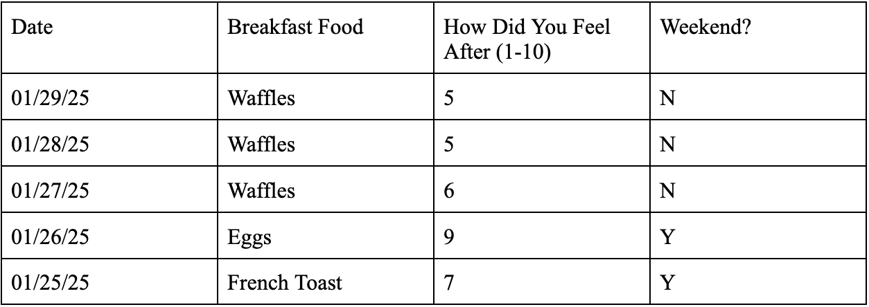
These tables aim to highlight how additional data makes modeling an outcome easier and increasingly accurate. The first table gives us decent data that narrows our options down to three potential breakfast foods. Having data on if the day falls on a weekend shows us that weekends may lead to additional time to make breakfast while the how did you feel after data may help rule out future cases in which the person’s breakfast made them ill.
In a nutshell, modeling any event tries to create a controlled environment to make predictions in. Said environment only knows the information that you choose to feed it, hence why predictive information is a core tenant of sound modeling. In Saverin’s case, he identified that having just historical oil prices wouldn’t suffice in giving apt estimates for day-to-day oil prices. He dug deeper and thought about the problem differently.
I recently found myself with a similar quandary to Saverin’s when creating a men’s college basketball (CBB) daily fantasy sports (DFS) projection model . On the surface, the problem seemed easy to me, but as I got into planning it, I quickly found myself questioning why events actually happen.
Often noted as sport’s most variance-laden game, college basketball has a unique make-up due to its year-over-year roster turnover and bifurcated scheduling. Roster turnover makes early season modeling a mess as the team’s dynamic doesn’t have a consistent prior starting point to base predictions off of. Additionally, the schedule gets split into two parts - non-conference and conference play. Non-conference play mostly has top teams as 20+ point favorites against bottom barrel Division I teams while conference play has teams with similar skill pitted against each other. These large swings in opponent skill level make it harder to create baselines for team/player skill.
To create this model, I first needed to understand what I wanted my final output to be which was a prediction for a player’s field goal makes, field goal attempts, three point field goal makes, three point field goal attempts, free throw makes, free throw attempts, points, offensive rebounds, defensive rebounds, assists, steals, blocks, and turnovers in a given matchup. To do this, I would need historical player data in addition to historical team-level data to provide context to a player’s matchup.
My methodology works from the top down, meaning I get player-level predictions by first generating team-level predictions and then divvying out those predictions based on a player’s historical outputs. Every individual stat I mentioned above, other than points, field goal, three point, and free throw makes, are initially modeled on a team-level. Rather than model points and makes on a team-level, I back into those numbers on a player-level by projecting their two-point and three-point field goal percentage as well as their free throw percentage independently and then multiply their percentage by the attempts prediction for each category, ultimately resulting in a points projection.
The features for each of these team-level models are different. For those not familiar, most modeling techniques rely on setting a target, the statistic you are trying to predict, and picking features that best predict that target. Features are simply statistics in your dataset that research has shown to be sound predictors of the target.
For the sake of example, let’s walk through the team-level defensive rebounding model. The features I chose for this model are the vegas-based team total, vegas-based opponent team total, and the spread. In addition to these statistics, I utilize multiple EWMAs for the team’s defensive rebounding rate, the opponent’s defensive rebounding rate allowed, the team’s rebounding totals, as well as a few others. EWMA stands for exponentially weighted moving average, a statistic where you assign a number as the “span” which shifts how much weight you put on more recent data points. Say you believe that the last few games are the most indicative of a team's rebounding prowess, you would put a very low span of 2-4, and if you thought results were relatively stable over time, the span would be in the 7-9 range. Setting EWMAs to low spans can lead to more accurate results according to mean absolute error, mean squared error, and R² but that can be a byproduct of overfitting data and results actually may be much worse when backtested. As we are deep into conference play at the time of writing, I have the span for the EWMAs across all my models set to 7.
From here, I feed these features into four different models for each target - XGBoost, Random Forest, Quantile Gradient Boosted Regression, and Bayesian Ridge. I then take the prediction from each of these models, assign a weight based on the model’s mean absolute error, mean squared error, and R², and divide them optimally to create an ensemble prediction.

The above screenshot shows the efficacy of each individual model when trying to predict team defensive rebounds as well as the ensemble that I use as my final prediction. The optimal weights in this case show that the optimal ensemble prediction ends up dropping the XGBoost entirely and my final prediction was the sum of:
(Random Forest prediction * .57) + (Gradient Boosting Prediction * .22) + (Bayesian Ridge prediction * .21)
Every model has different optimal weighting and every model clearly shows improved performance by the ensemble compared to any individual model.
The quality of your data directly correlates to the results of your model. My team-level models all have an R² ranging from .4 to .55, meaning that 40% to 55% of the target’s variance can be explained by my models. College basketball doesn’t have the best publicly available data, making it tough to create extremely predictive models. I think that this lack of data leads the public to believe college basketball has higher outcome variance than it truly does.
In an ideal world, a model would be created with the most granular data possible. Synergy houses this data, but unfortunately only sells it to teams and media. The best way to predict two point field goal attempts, for example, isn’t to look at past two point field goal attempts that previous box scores show. The best way would be to predict each type of two point field goal attempt and then sum them up. For example, Team A and Team B both allow, on average, thirty two-point-field-goal attempts per game to their opponents. On the surface, these teams have similar tendencies. Digging deeper, 70% of Team A’s two point attempts come from post ups, 20% come from off-the-dribble mid-range jumpers, and the remaining 10% come from floaters. Team B only allows 20% of its two point attempts from post-ups due to a strong post defender while the remaining 80% come from off-the-dribble mid-range jumpers. These two teams by my model’s current logic are the exact same, but more granular data shows that they are drastically different.
These distinctions become increasingly important when doling out stats on a player-level. On paper, a plus two-point field goal attempt matchup for a big may actually be better for the guard on his team because the opposing team plays drop coverage which historically leads to an increased amount of two-point jumpers by the pick-and-roll ball handler.
Back to the model’s inner-workings -
After predicting all the team-level statistics, it’s time to spread these predictions across the players on a given fantasy slate. I start by inputting a file with minute projections for each player. I project minutes by hand because it’s a nuanced art that can be influenced by game score, matchups, and coachspeak. It’s difficult to project minutes in the first place and even more difficult to model like you would a traditional stat such as defensive rebounds, steals, or assists.
I then feed this data frame into a simulator. When I first created my model, I used the same team-level ensemble methodology on the player-level which led to extremely poor results as the model was overfitting data. This led me to using a simulator, which doles out the predicted team-level stats across 10,000 simulations, resulting in an average for each player. Decay factors are also fed in, giving the simulator instructions on how to weigh historical data. I use the “random walk” equation for calculating decay weights: 1 / (games_ago + intercept). Every stat has a different intercept as certain stats are more stable over time. Interestingly, Mike Beuoy’s power rankings methodology, the inspiration for using the random walk equation, estimates the intercept for NBA as 1.5 and 0.5 for NCAAB (on the team-level) while backtesting past projections estimated the optimal intercepts in the range of 1-1.2 for my player-level simulator.
My output ends up looking like this:

Although this approach produces results that have been better than all publicly available CBB DFS projections, it still has its pitfalls. The modeling techniques used have a tendency to smooth past results and err towards mean outcomes. This has my model poorly predicting certain extreme game environments. Some of the best examples are teams against Houston or Alabama. Houston notoriously yields team totals in the 50s when at home, a far cry from the mid 60s to 70s totals we typically see. My model tends to boost Houston’s opponents seven to eight points over their implied team total, an error most likely caused by the opposing team not having ample historical data in similar game environments. Alabama game environments are the opposite where they play with such pace that my model typically under projects their opponent relative to the team’s implied total.
This ultimately highlights the importance of interpreting the model’s results. After my initial run, I sum player-level points to make sure that I’m somewhat close to the market’s team-level points projection. Additionally, I’ll cross-check my numbers with player lines on Underdog and DraftKings Sportsbook to make sure I’m not taking any outsized positions. If I notice any massive discrepancies I’ll manually go in and adjust my final outputs.
Although my model isn’t error-free, simply having control over my entire process and seeing final outputs granularly allows me to make more informed adjustments. Current publicly available projections just give the final fantasy projection, making it hard to know how aligned to the market they are. I’ll oftentimes find my projection lower than all market sources while still being higher than the Vegas team total. Players on these teams are usually ones I stay away from as the field’s understanding greatly differs from the market’s game environment prediction.
Along the road of predicting outcomes, you’ll find that a model serves as a guide. Numbers without context are simply noise. Public projections are amazing resources, but any bettor’s edge is knowing how to weigh different bits of information and if you have no idea what the inputs of a projection system are, you cannot be sure you aren’t double counting something the system already has accounted for. Markets and DFS contest fields already have a lot of information accounted for as a collective and if you choose to play in those fields you must attempt to try to know something the field or market does not.
Simply put, thinking about problems differently reaps larger benefits than aligning with the status quo. Be it Eduardo Saverin predicting oil prices, someone predicting what you had for breakfast, or trying to figure out what college basketball players will perform well today, you stand to gain more by understanding what everyone else is doing and figuring out the optimal way to deviate. As college hoops become more skill-based in understanding available transfers’ possible fit and development curve, the benefits of thinking differently will be exacerbated. Everyday we all play games of limited, imperfect information and it’s up to us to weigh this limited information to our benefit. And if you believe thinking different isn’t all that and you don’t believe Eduardo or I, ask Apple: